ipython notebooks in 15 minutes

This introduction to the use of ipython notebooks assumes that you have already done a Python installation which includes a current version of ipython (e.g. Enthought) and that you are familiar with the basics of the Python language.

ipython notebooks provide a web browser interface to the ipython Python interpreter. They work through an ordinary web browser of your choice. An ipython notebook document also allows you to interweave formatted text (including mathematical equations) and graphics with executable and editable Python code. Notebooks provide an ideal platform for writing documents which both explain concepts and allow the reader to interact with the calculations and even rewrite code. This is invaluable both for pedagogical purposes and for communicating research results.

Since ipython notebooks incorporate quite powerful editing capabilities, the notebook server may be the only interface to Python you ever need. It could well substitute for integrated development environments (e.g. Canopy) for all but the most elaborate and complex projects.

First start up the notebook server

This example shows you how to start up a notebook server on your own computer. Later we'll show how to start up and use a notebook server running on a remote computer which you can access over the network.

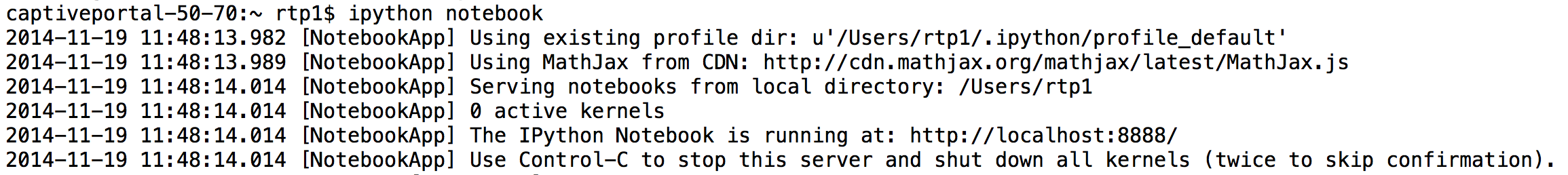
Open a command line window and type in the command ipython notebook . Here is what the result looks like in the Mac OS X Terminal window. It will look somewhat different for other operating systems. The command will produce some output telling you things about the server, which you can ignore for now. It may also spit out a few error messages, most of which are probably harmless.

The server will launch your default web browser (if necessary) and open a browser window landing you in the Notebook dashboard page:

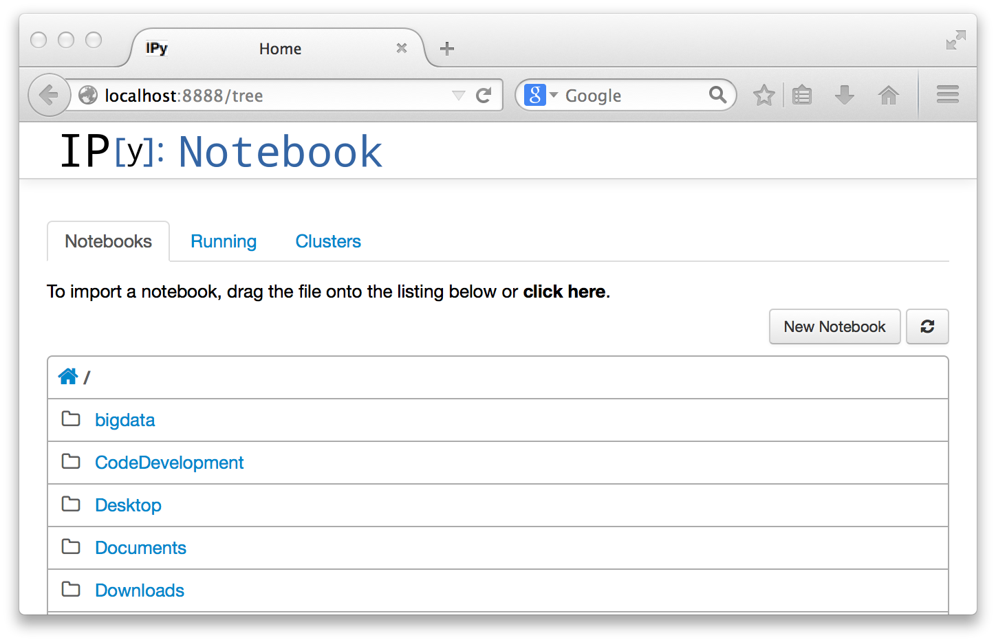
The Notebooks tab of the dashboard (all we need for now) is just a way to navigate your directories. The home (little house) icon is your home directory, and you see your other directories (folders), and can navigate to any of them by clicking on the diretory name. If you already had a notebook document stored, you could just open it by clicking on it.

Create a new notebook and do some python

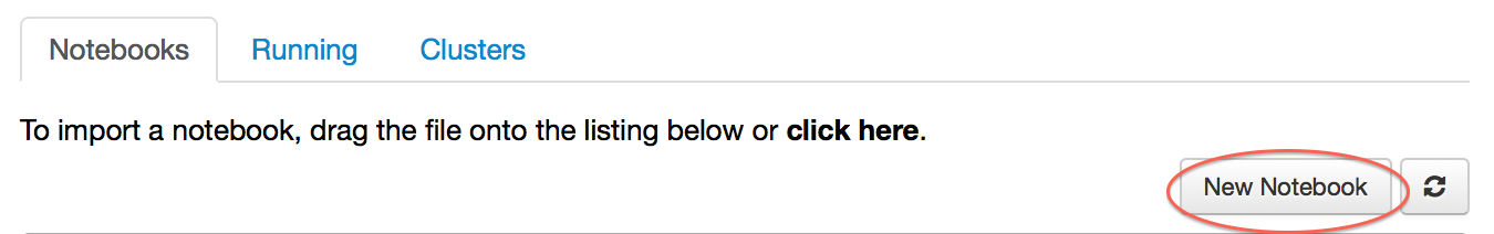
But lets say you don't have any notebooks, or want to create a new one. First navigate to the directory where you want your notebook to be stored, then created a new notebook by clicking on the New Notebook button, circled below.

 

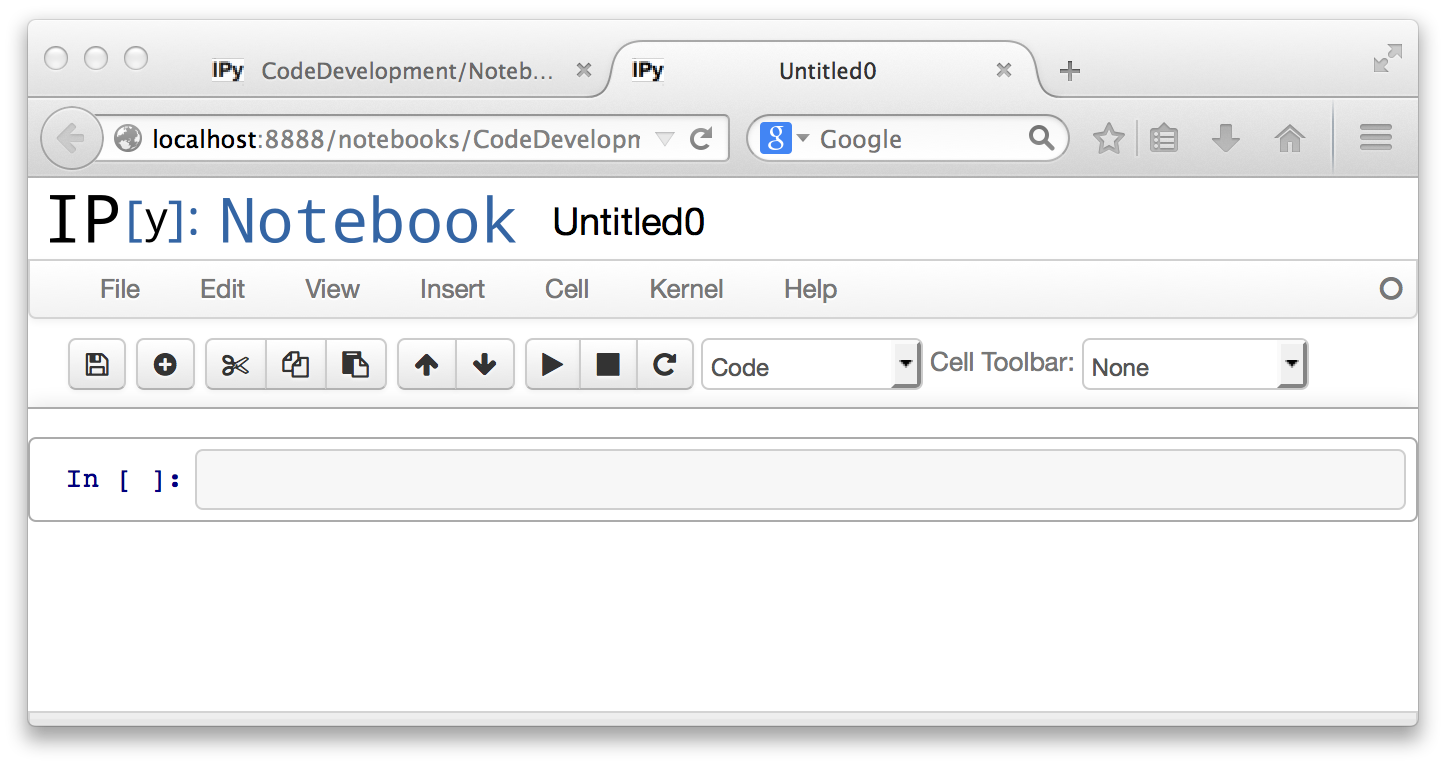
This will create a new notebook documentt. The notebook is displayed under its name in a new tab of the browser window. The notebook document is automatically saved, with a name picked by the server. You can rename the document at any time using the File menu. A notebook document consists of a series of "cells," which can process various kinds of contents. The fresh notebook comes up with a single cell, which is a code cell.

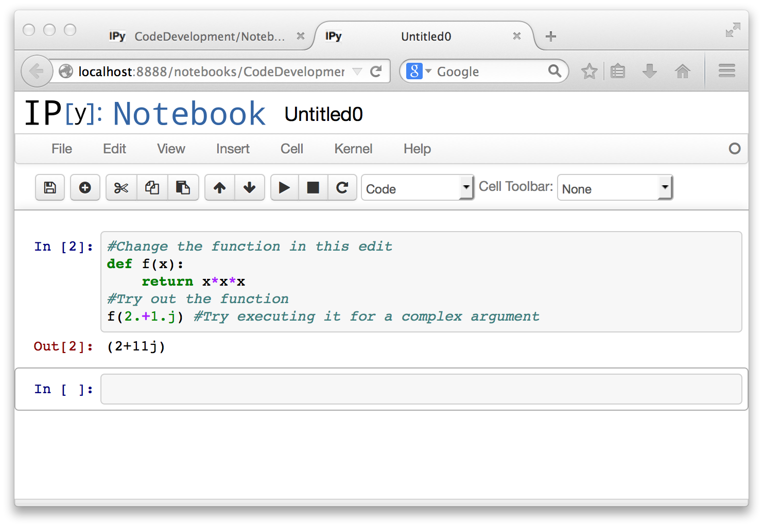
You can type any number of lines of Python into a code cell, and edit it within your Browser. The Editor is Python aware, and automatically does indentation and colorization. Below, we have typed a function definition into the cell, and also a line to execute the function for a specified value.

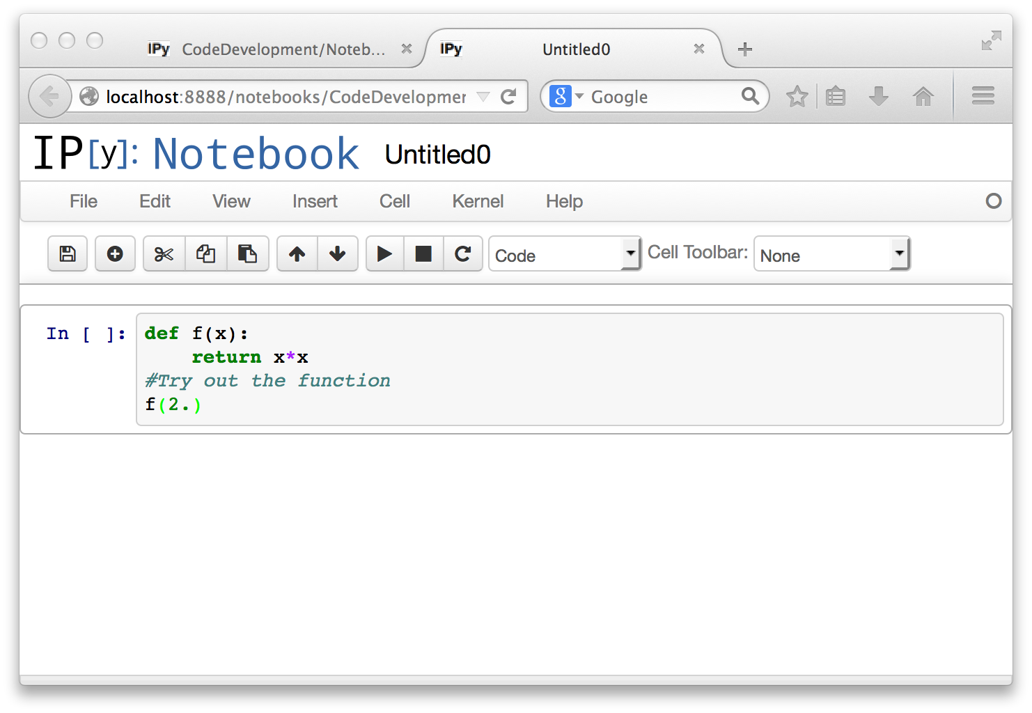
Unlike what happens in a command line interpreter session, the code you type in does not execute as soon as the statements are complete. You execute the Python code in the cell, using the circled right-triangle button. The keyboard shortcut for executing a cell is option-<return> on a Mac, and keyboard shortcuts exist on other systems as well. Here is the result of executing the cell.

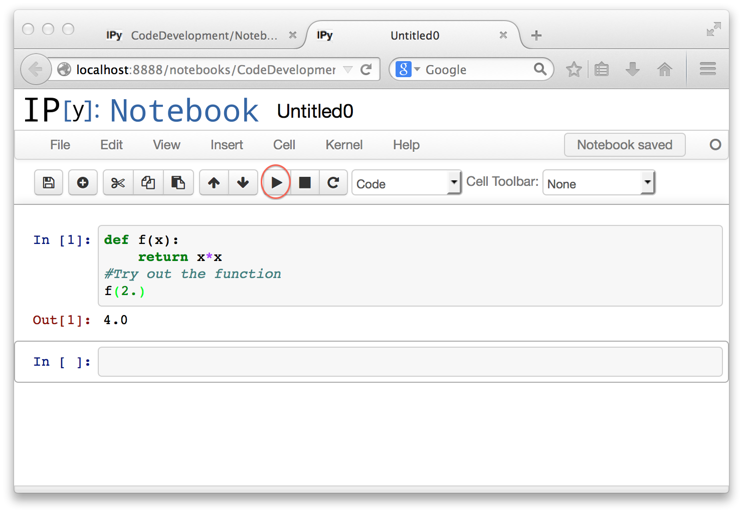
The execution has produced some output, but it has also defined the function, which you can then use in subsequent code cells. By default, execution creates a new code cell that you can type more stuff into. You can also edit any code cell and then execute it again to see the new result.

Re-executing a code cell does not create a new code cell. It does change the index in the square brackets in In[...] and Out[...], just as in the command line ipython interpreter.

The items in the Insert and Edit menus give you ways to move around cells and merge or split them. Most of the menu items are pretty self-explanatory. You can play around with them to see how they work.

Make a plot of some results

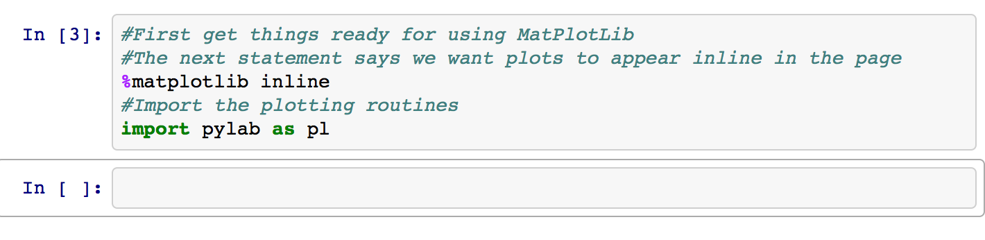
You can perform Python operations that create graphical output from within a notebook. Ordinarily, such operations will create a separate graphics window of their own, which is not handled by your web browser. However, if using any graphics package based on MatPlotLib, you have the option of specifying that graphics be displayed inline in the notebook page. This is done via the %matplotlib inline magic command. Inline graphics will be saved together with the rest of your notebook. Here is how you set things up to use MatPlotLib, with the inline option.

And here we are creating a plot:

 

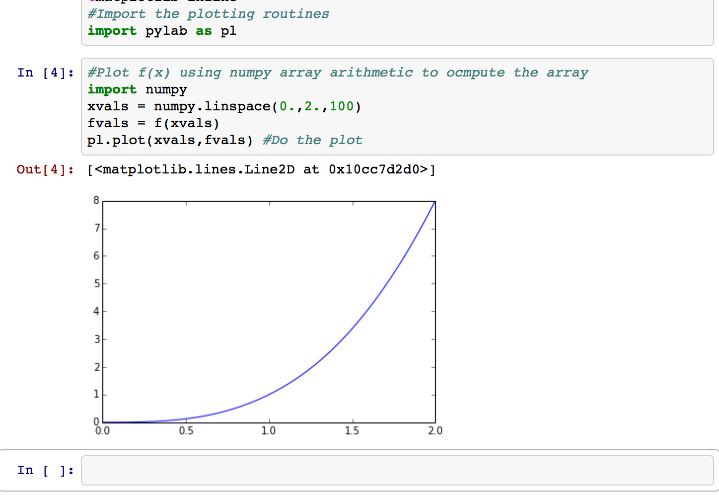
Note that the function f(x) defined in a previous cell (once that cell was executed) is still available, since each notebook runs in a single interpreter session ("kernel") until the kernel is restarted. If the kernel is restarted, any cell whose results you want would need to be executed again.

Other kinds of cells

Notebooks support other types of cells besides Code cells. The type of cell is chosen via the pop-up menu on the toolbar, which by default is set to Code . The chief use of the other types of cells is to allow a notebook to incorporate formatted text and graphics that give the document organization, provide mathematical background, document code, and give instructions or suggestions to the user. Header cells are used to divide a document up into topics, and come in a choice of different levels. Markdown cells are the most versatile, and can contain a variety of text formatting commands (including LaTeX) and html codes. Graphics can be incorporated through html . Here is an example of a notebook with heading and markdown cells before it is executed. The first markdown cell is highlighted, together with the menu item used to select its type.

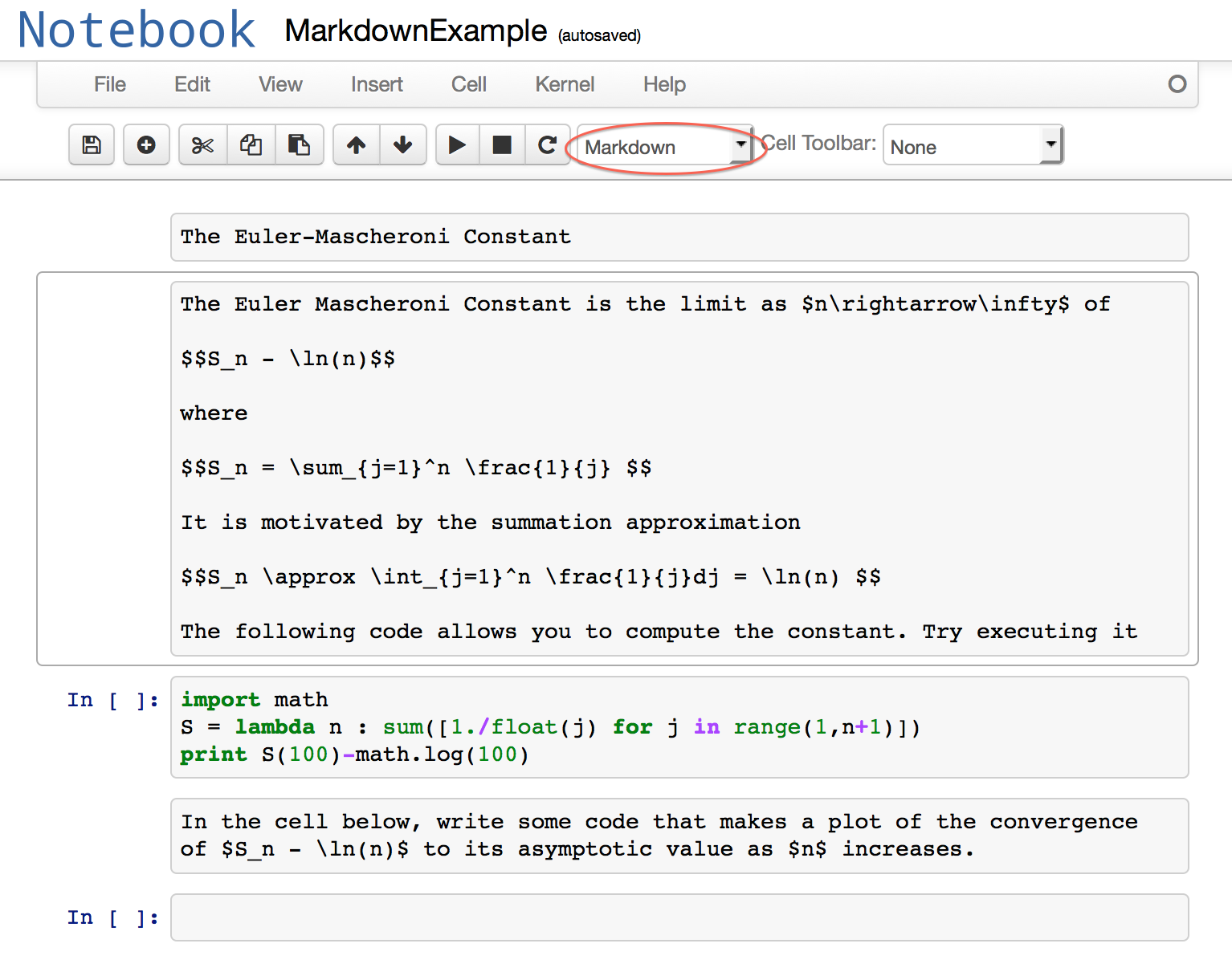
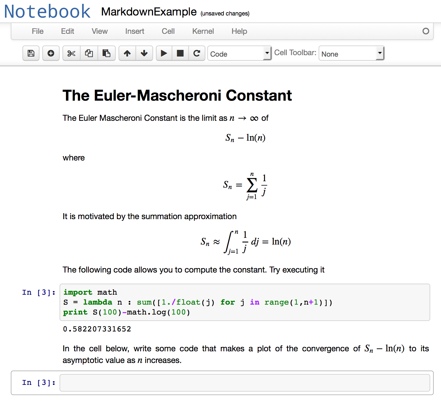
The header and markdown cells are executed in the same way as a code cell, but instead of producing output produce the formatted text and graphics. Here is what the notebook looks like after everything has been executed.

If you want to get the raw text of a markdown or header cell back so you can edit it, you just double click on the cell.

Put away your toys

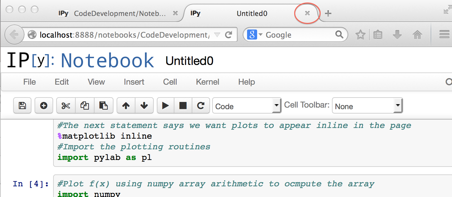
When you are done with your notebook, you can just close the notebook tab with the go-away box as you would for any other browser tab, and you will wind up back at the dashboard (you can also tab back to the dashboard at any time to open other notebooks).

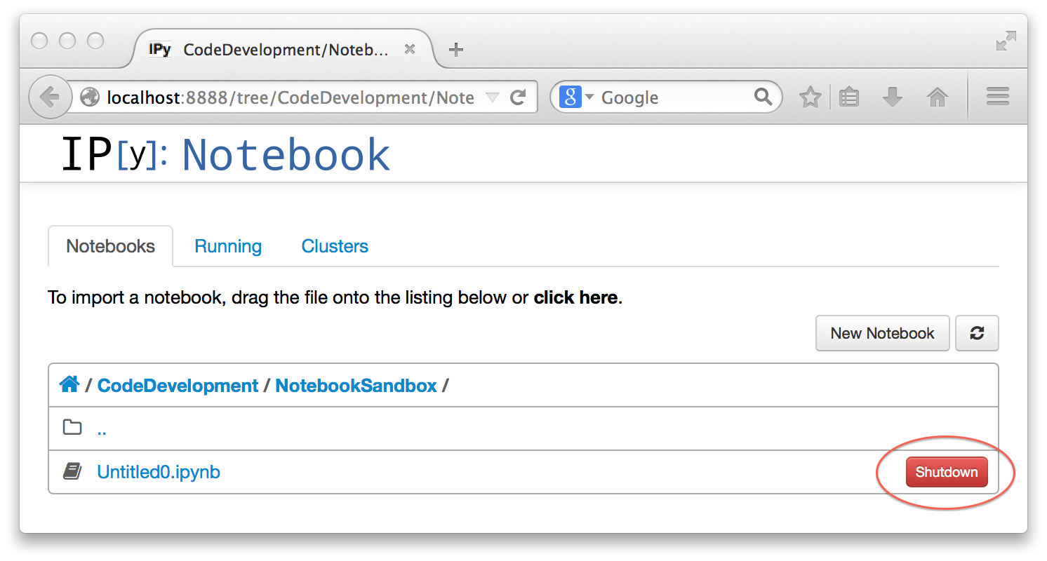
The listing of notebooks on the dashboard will have a shutdown button which allows you to shutdown the notebook's terminal session, which you would ordinarily do if you aren't planning to work with the notebook again soon. This doesn't delete the notebook; it is still there and you can re-open it later and do more work on it. However, any code cells that produce results you need in later code cells (e.g. function definitions or calculated values) will need to be re-executed. If you don't shutdown the notebook, you can resume where you left off by just re-opening the notebook, without the need to re-execute anything.

You can also close and shutdown a notebook all in one step from the File menu.

Once you have shut down your notebooks, you still haven't shut down the notebook server, even if you close all your windows and quit your browser. The server is still waiting to server you whenever you need it, and to reconnect, you just need to point your browser to the server's URL. There really isn't any good reason to ever shut down the notebook server (just put away the terminal window instead, so it isn't in your way), but if you do want to shut it down, you do that cleanly by going back to the terminal window and typing control-c once, then responding to the shutdown prompt:

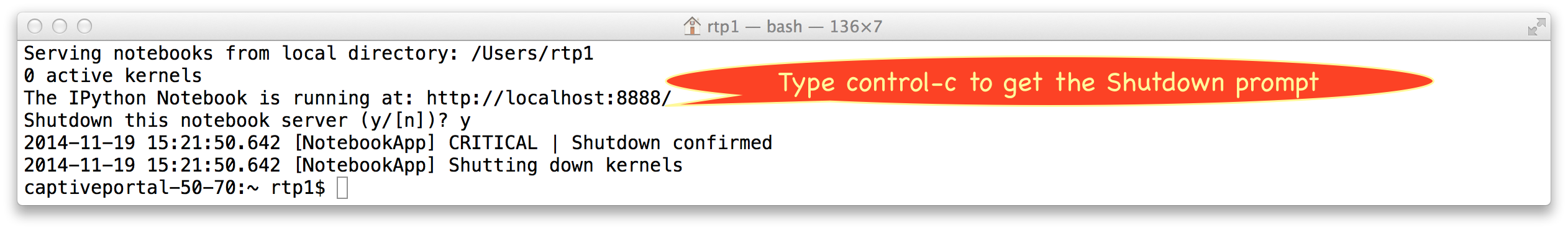
Alternately, you can do it faster by typing control-c twice in a row quickly.

How to start and use a remote notebook server

This section provides some specialized information that probably goes beyond the "fifteen minute" limit. Most users will be running the notebook server on the same computer that is running their web browser, and so will not need to know how to connect to a notebook server over the network. The term localhost in the URL for the server in fact means that the browser is connecting to a process on the local machine. However, there are circumstances where it may be desirable to use your web browser to connect to a notebook server running on a remote machine, via the network.

The instructions to follow assume you have an account on the remote Linux or Mac computer, which we'll call borta.somewhere.els . Let's suppose your userid on this machine is mymble . The instructions also suppose that your account has been set up to use ipython . For the Enthought Canopy distribution, this may mean you need to execute the Canopy app using the full master-install pathname before the first time you use ipython, to set up your local environment. You only need to do this one time. It is also possible for the administrator of the remote machine to set up a public notebook server that can be accessed directly via a web browser without the user needing an account, but the following instructions show you how to set up your own private notebook server. Private servers involve fewer security issues, and also make it more straightforward to store your work where it won't get mixed up with that of other users.

The general procedure is to log on to the remote machine, start up your own personal notebook server there, and then connect to it by establishing a "tunnel" that allows a browser running on your local machine to connect to the remote notebook server as if it were running locally. Establishing the tunnel requires a second logon, using the ssh command from a terminal window on your local machine (or an ssh app on Windows). For Windows, the usual ssh app is putty .

First you log in to the remote machine using the command

ssh mymble@borta.somewhere.els

in a terminal window, with the userid and remote computer name replaced by your own values. (On Windows you'd probably be using the putty-ssh terminal app instead). After issuing the command, you'll get a password prompt. Enter your password to log in. Then you start up a notebook server using the command

ipython notebook --no-browser

The --no-browser option tells ipython not to start up a web browser on the remote machine. (You don't need the browser on the remote machine since you'll be using your local browser, and if you are logging in without an x11 graphical connection an attempt to open a browser window might create problems). The command will give you the same kind of startup information you'd get if starting up a notebook server locally. The output will look something like this:

2014-11-22 10:09:45.602 [NotebookApp] Using existing profile dir: u'/Users/rtp1/.ipython/profile_default'
2014-11-22 10:09:45.610 [NotebookApp] Using MathJax from CDN: http://cdn.mathjax.org/mathjax/latest/MathJax.js
2014-11-22 10:09:45.632 [NotebookApp] The port 8888 is already in use, trying another random port.
2014-11-22 10:09:45.633 [NotebookApp] Serving notebooks from local directory: /Users/rtp1
2014-11-22 10:09:45.633 [NotebookApp] 0 active kernels
2014-11-22 10:09:45.633 [NotebookApp] The IPython Notebook is running at: http://localhost:8889/

The important thing to note is the last line shown above, which shows the URL under which the notebook server is running. In this case, a notebook server with "port number" 8888 is already in use, so the new notebook server is created with port number 8889 to keep it straight from the other one.

But you can't just put the URL http://localhost:8889/ into your local browser and have it work, since that will look for a process running on your local machine. Instead, you must create a "tunnel" that connects a local URL with the remote one. This is also done in ssh, and requires a second ssh login to the remote machine. Open a new terminal window (on Mac or Linux) and type in the command:

ssh mymble@borta.somewhere.els -L8890:localhost:8889

where the number 8890 in the example can be replaced by any port number on the local machine that is not in use, and the number 8889 should be replaced by the port number under which the remote notebook server is actually running. You should again replace the userid and remote computer name by your actual values. You will get another password prompt, to which you respond. Instructions for how to set up an ssh tunnel with the putty app on Windows are widely available on the web, e.g. here.

Now, all you need to do is open a browser window on your local machine and point it to the URL http://localhost:8890 (or whatever local port number you chose). After that, you can just use the notebooks exactly as if the server were running on your local machine. Any notebooks and output you produce will be stored in your home directory on the remote machine (or a subdirectory, if you have created one for the purpose).

When you are done, shut down the notebook and server in the usual way. Then log out of both of your ssh sessions.

When running notebooks on a remote server, it is recommended that graphics be done inline so that graphical display is handled by your web browser. If you don't specify inline graphics, the graphics window created by the graphics package will generally not be handled by your web browser, so you need to have an x11 connection (such as provided by the xquartz terminal app on a Mac or the default terminal on Linux) that allows a remote machine to put up graphics on your screen.

Depending on how up-to-date the operating on the remote system is, you might get an error message concerning some missing libraries (usually the libpng family) when you try to import matplotlib or pylab . If you run into this problem, you can fix it easily by running the Canopy app on the remote machine and clicking on the Package Manager button, which allows you to easily install new packages in your personal Python environment with a single click. However, to run the Canopy app on a remote machine, you need to be logged in using an x11 (e.g. xQuartz on a Mac) terminal. If you are using a Windows computer to access the remote machine, it is probably easier to get somebody with a Mac or Linux machine to access your account and do the install for you, since it only needs to be done once and after that you don't need x11 if you are going to interact with the remote machine using just notebooks.